Autoencoders

Training deep neural networks (i.e., networks with several hidden layers) is challenging, because normal training easily gets stuck in undesired local optima. This prevents the lower layers from learning useful features. This problem can be partially circumvented by pre-training the layers in an unsupervised fashion and thereby initialising them in a region of the error function which is easier to train (or fine-tune) using steepest descent techniques.

One of these unsupervised learning techniques are autoencoders. An autoencoder is a feed forward neural network which is trained to map its input to itself via the representation formed by the hidden units. The optimisation problem for input data \(\vec{x}_1,\dots,\vec{x}_N\) is stated as:

\[\min_{\theta} \frac 1 N \sum_{i=1}^N (\vec x_i - f_{\theta}(\vec x_i)^2 \enspace .\]

Of course, without any constraints this is a simple task as the model will just try to learn the identity. It becomes a bit more challenging when we restrict the size of the intermediate representation (i.e., the number of hidden units). An image with several hundred input points can not be squeezed in a representation of a few hidden neurons. Thus, it is assumed that this intermediate representation learns something meaningful about the problem. Of course, using this simple technique only works if the number of hidden neurons is smaller than the number of dimensions of the image. We need more advanced regularisation techniques, like dropout to work with overcomplete representations (i.e., if the size of the intermediate representation is larger than the input dimension). But especially for images it is obvious that a good intermediate representation must be somehow more complex: the number of objects that can be seen on an image is larger than the number of its pixels.

As a dataset for this tutorial, we use a subset of the MNIST dataset which needs to be unzipped first. It can be found in examples/Supervised/data/mnist_subset.zip.

The following includes are needed for this tutorial:

#include <shark/Data/Pgm.h> //for exporting the learned filters
#include <shark/Data/SparseData.h>//for reading in the images as sparseData/Libsvm format
#include <shark/Models/LinearModel.h>//single dense layer
#include <shark/Models/ConcatenatedModel.h>//for stacking layers
#include <shark/ObjectiveFunctions/ErrorFunction.h> //the error function for minibatch training
#include <shark/Algorithms/GradientDescent/Adam.h>// The Adam optimization algorithm
#include <shark/ObjectiveFunctions/Loss/SquaredLoss.h> // squared loss used for regression
#include <shark/ObjectiveFunctions/Regularizer.h> //L2 regulariziation

Training autoencoders

Training an autoencoder is straight forward in shark. We just setup two neural networks, one for encoding and one for decoding. Those are then concatenated to form one autoencoder network:

//We use a dense lienar model with rectifier activations
typedef LinearModel<RealVector, RectifierNeuron> DenseLayer;

//build encoder network
DenseLayer encoder1(inputs,hidden1);
DenseLayer encoder2(encoder1.outputShape(),hidden2);
auto encoder = encoder1 >> encoder2;

//build decoder network
DenseLayer decoder1(encoder2.outputShape(), encoder2.inputShape());
DenseLayer decoder2(encoder1.outputShape(), encoder1.inputShape());
auto decoder = decoder1 >> decoder2;

//Setup autoencoder model
auto autoencoder = encoder >> decoder;
//we have not implemented the derivatives of the noise model which turns the
//whole composite model to be not differentiable. we fix this by not optimizing the noise model
autoencoder.enableModelOptimization(0,false);

Note that for the deeper layers we use the shape of the output of the previous layers (in this case just a 1-d shape with the number of neurons) to specify the shape of the input of the next layer.

Next, we set up the objective function. This should by now be looking quite familiar. We set up an ErrorFunction with the model and the squared loss. Here we enable minibatch training to speed up the training progress. We create the LabeledData object from the input data by setting the labels to be the same as the inputs. Finally we add two-norm regularisation by creating an instance of the TwoNormRegularizer class:

//create the objective function as a regression problem
LabeledData<RealVector,RealVector> trainSet(data.inputs(),data.inputs());//labels identical to inputs
SquaredLoss<RealVector> loss;
ErrorFunction error(trainSet, &autoencoder, &loss, true);//we enable minibatch learning
TwoNormRegularizer regularizer(error.numberOfVariables());
error.setRegularizer(regularisation,&regularizer);
initRandomNormal(autoencoder,0.01);

Lastly, we optimize the objective using Adam:

Adam optimizer;
error.init();
optimizer.init(error);
std::cout<<"Optimizing model "<<std::endl;
for(std::size_t i = 0; i != iterations; ++i){
        optimizer.step(error);
        if(i  % 100 == 0)
                std::cout<<i<<" "<<optimizer.solution().value<<std::endl;
}
autoencoder.setParameterVector(optimizer.solution().point);

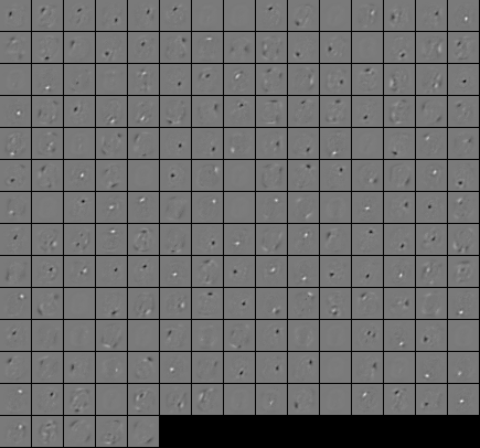
Visualizing the autoencoder

After training the different architectures, we printed the feature maps of the first layer (i.e., the input weights of the hidden neurons ordered according to the pixels they are connected to). Let’s have a look.

exportFiltersToPGMGrid(“features”,encoder1.matrix(),28,28);

Full example program

The full example program is AutoEncoderTutorial.cpp.

Attention

The settings of the parameters of the program will reproduce the filters. However the program takes some time to run! This might be too long for weaker machines.