Principal Component Analysis

Background

Principal component analysis (PCA), also known as Karhunen-Loeve transform, is arguably the most fundamental technique in unUnsupervised learning. It is frequently used for (linear) dimensionality reduction, (lossy) data compression, feature extraction, and data visualization. Let us consider a set of l data points

\[S=\{x_1,\dots, x_l\} .\]

Let n real-valued attributes (n features) represent a single data point. How can we reduce the length of the description to m < n variables such that as much information as possible is preserved? How many dimensions are needed to capture a certain percentage of the variability of the data? These are typical questions that arise when we want to do dimensionality reduction, feature selection, and compression (these three terms usually refer to similar processes, emphasizing different aspects of the same algorithmic procedure). Dimensionality reduction is closely linked to visualization. When visualizing high-dimensional data, the question arises of how to project the data to two or three dimensions such that the visualization of these dimensions reflects as much of the variability of the data as possible. Principle component analysis gives (under particular assumptions) answers to these questions.

The goal of PCA is to find an m-dimensional affine linear model of the n-dimensional data points in S that represents the original data as accurately as possible in a least-squares sense. This model does not only minimize the reconstruction error when mapping the data back to the original space, it is also the affine linear model that yields the representation that maximizes the overall variance when encoding the points in S using only m dimensions. For details see for instance [DMLN5].

PCA in Shark

The following includes are needed for this tutorial:

#include <shark/Algorithms/Trainers/PCA.h>
#include <shark/Data/Pgm.h>

Face recognition problem

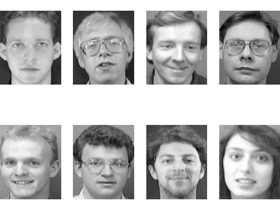
As a classical example for PCA, let us consider computing eigenfaces [TurkPentland1991] using the Cambridge Face Database [SamariaHarter1994] as an example. It contains 92x122 images of frontal faces, some examples are shown in Figure 5.2. We can represent each face by a vector by inflating the image, that is, by concatenating the image rows. Although the images are rather small, we get a 10304-dimensional representation (i.e., n = 10304). That is, in the original representation 10304 basis vectors, one for each pixel, define the image space. Principal component analysis can help us to significantly reduce the description length of the images.

The data can be downloaded from here. Some sample faces are shown in the following figure.

Reading in the data

First, let us read in the data. There is a function for recursively scanning a directory for images in pgm format and reading them in:

const char *facedirectory = "Cambridge_FaceDB"; //< set this to the directory containing the face database
UnlabeledData<RealVector> images;

        importPGMSet(facedirectory, images);

unsigned l = images.numberOfElements();   // number of samples
unsigned x = images.shape()[1]; // width of images
unsigned y = images.shape()[0]; // height of images

The imagesInfo struct contains sizes and names of the individual images.

Models and learning algorithm

Doing a PCA is as simple as:

PCA pca(images);

Karhunen-Loeve transformations are affine linear models. For encoding data to an m-dimensional subspace we use:

unsigned m = 299;
LinearModel<> enc;
pca.encoder(enc, m);

The last line encodes (i.e., represents in the PCA coordinate system) the whole image database.

We can easily map from the m dimensional space back to the original n dimensional space by the optimal linear reconstruction (the decoder):

LinearModel<> dec;
pca.decoder(dec, m);

For instance, let us reconstruct the following first image using just the first m=300 components.

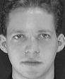
Then we write

unsigned sampleImage = 0;

boost::format fmterRec("facesReconstruction%d-%d.pgm");
exportPGM((fmterRec % sampleImage % m).str().c_str(), dec(encodedImages.element(sampleImage)), x, y);

and get the following image.

Further evaluation of the model

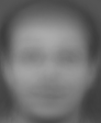
We can retrieve the eigenvalues and eigenvectors of the model by calling pca.eigenvalues() and pca.eigenvectors(), respectively. The number of eigenvalues and eigenvectors returned by these functions is min(l, n). The eigenvalue i can also be retrieved by pca.eigenvalue(i). Visualizing the mean face is done by

exportPGM("facesMean.pgm", pca.mean(), x, y);

resulting in the following mean image.

Full example program

An extended eigenface example program is PCATutorial.cpp. The face database can be downloaded from here.

Additional features

The Shark PCA automatically applies the “more attributes than data points” trick, see [DMLN5]. It easily allows for “whitening”, that is, learning a transformation giving unit variance of the sample data in the new coordinate system along each component.

As always, please look at the file documentation, the example programs, and the unit test (Test/Algorithms/Trainers subdirectory).

References

[DMLN5]

(1, 2) C. Igel. Data Mining: Lecture Notes, chapter 5, 2011

[SamariaHarter1994]

F. Samaria and A. Harter. Parameterisation of a stochastic model for human face identification. In IEEE Workshop on Applications of Computer Vision, pages 138-142. IEEE Computer Society Press, 1994.

[TurkPentland1991]

M. Turk and A. Pentland. Eigenfaces for recognition. Journal of Cognitive Neuroscience, 3(1):71-86, 1991.